


Building a basic neural network
A simple task for a simple model
Our first artificial neural network will be simple, and it therefore needs a simple task to be trained on. We will train it to classify numbers between 0 and 1 as being either less than 0.5 (category 0) or equal to, or higher than, 0.5 (category 1). Phrased differently, we're going to teach the network to round numbers between 0 and 1.
Generating the data
We first generate an array of 10,000 random numbers (between 0 and 1), which we will use as the training data (or: input) for the model; that is, each training observation consists of a single number.
np.random.random(10000) returns a one-dimensional array of shape (10000,). However, we need a two-dimensional array for our model. Specifically, the first axis should correspond to the individual observations, and should therefore be of length 10,000. The second axis should correspond to the values from each individual observation, and should therefore be of length 1. We can accomplish this by explicitly changing the shape of data to (10000, 1).
import numpy as np

data = np.random.random(10000)
data.shape = 10000, 1
print(data[:5])  # Look at the first five observations
Output:
[[0.87777315]
 [0.96180321]
 [0.61156799]
 [0.44780278]
 [0.06562224]]
Next, we check which numbers in the training data are larger than, or equal to, 0.5. This results in an array of boolean values (True or False), which we turn into an array of int (1 or 0) values. This array will serve as the labels (or: expected output) for our model.
labels = np.array(data >= .5, dtype=int)
print(labels[:5])  # Look at the first five labels
Output:
[[1]
 [1]
 [1]
 [0]
 [0]]
Building a simple model
The Sequential model class allows you to specify a model's architecture as a list (or: sequence, hence the name) of layers. We specify two layers, both of which are Dense, which means that each neuron in the layer is connected to all neurons in the layer above.
The first (non-input) layer, which consists of 8 neurons, specifies the shape of the input observations, which in our case is only a single number (i.e., an array of shape (1, )). The activation keyword specifies how the neurons translate their input to an output. Here we use the rectified-linear-unit function ('relu'), which essentially means that neurons cannot have a negative output.
The second layer, which consists of two neurons, is our output layer. The 'softmax' activation function essentially means that the neuron's output is squashed into the 0 - 1 range.
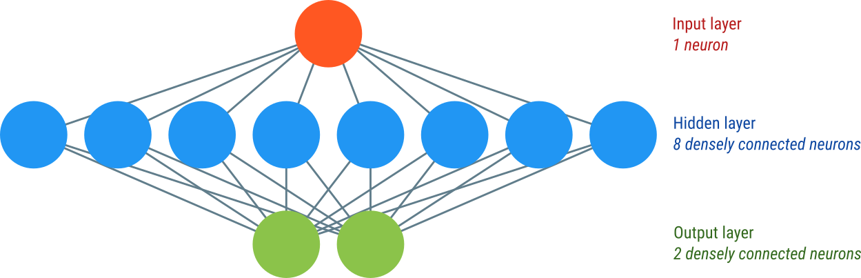
Figure 1. Our network consists of an input layer, a hidden layer, and an output layer.
It is common to think of the input as a layer as well, even though it is not specified as such in Keras. We can therefore think of our model as a three-layer network, with one input layer (consisting of one neuron), one hidden layer (consisting of eight neurons), and one output layer (consisting of two neurons). A layer is referred to as 'hidden' if it's neither an input layer nor an output layer.
from keras import Sequential
from keras.layers import Dense

model = Sequential([
    Dense(units=8, input_shape=(1,), activation='relu'),
    Dense(units=2, activation='softmax'),
])
Next, we compile the model so that it's ready to be trained. In doing so, we need to specify three things.
The optimizer keyword specifies the algorithm that will be used to adjust the weights in the model. We will use Adam, but other algorithms are available as well, and the choice of one algorithm over another is largely one of preference and experience.
The loss keyword specifies the loss function, which is the algorithm that determines how wrong the model's predictions are. The goal of training is to reduce the loss. We will use sparse categorical crossentropy, which assumes that label values of 0 mean that the first neuron in the output layer should be the most active, whereas label values of 1 mean that the second neuron should be the most active.
The accuracy keyword specifies a metric that is printed during training so that you have some idea of how well the model is performing. This is just for visualization and doesn't affect the training process itself.
model.compile(
    optimizer='adam',
    loss='sparse_categorical_crossentropy',
    metrics=['accuracy']
)
Now let's look at the model summary:
model.summary()
Output:
Model: "sequential"
_________________________________________________________________
 Layer (type)                Output Shape              Param #
=================================================================
 dense (Dense)               (None, 8)                 16

 dense_1 (Dense)             (None, 2)                 18

=================================================================
Total params: 34
Trainable params: 34
Non-trainable params: 0
_________________________________________________________________
Our model has 34 parameters, which correspond to all the weights of the connections between the neurons, as well as the bias parameter for each neuron (a kind of baseline level of activity that a neuron has in the absence of any input).
The first layer consists of eight neurons, which each have one connection to the input neuron plus one bias, so 8 × (1 + 1) = 16 parameters in total. The second layer consists of two neurons, which each have one connection all eight neurons in the preceding layer plus one bias, so 2 × (8 + 1) = 18 parameters in total.
Training the model
To train the model, we simply call the fit() function. During training, the model's 34 parameters are adjusted to minimize the loss.
The epochs keyword specifies how often the training data should be used to fit the model. In our case, we specify 10 epochs, which is similar to calling fit() 10 times in a row with the same data and labels.
The verbose keyword specifies how much information should be printed out during training.
model.fit(x=data, y=labels, epochs=10, verbose=2)
Output:
Epoch 1/10
313/313 - 0s - loss: 0.4922 - accuracy: 0.7621 - 420ms/epoch - 1ms/step
Epoch 2/10
313/313 - 0s - loss: 0.3087 - accuracy: 0.9424 - 175ms/epoch - 560us/step
Epoch 3/10
313/313 - 0s - loss: 0.2037 - accuracy: 0.9800 - 170ms/epoch - 544us/step
Epoch 4/10
313/313 - 0s - loss: 0.1509 - accuracy: 0.9915 - 170ms/epoch - 542us/step
Epoch 5/10
313/313 - 0s - loss: 0.1214 - accuracy: 0.9953 - 180ms/epoch - 575us/step
Epoch 6/10
313/313 - 0s - loss: 0.1025 - accuracy: 0.9966 - 189ms/epoch - 604us/step
Epoch 7/10
313/313 - 0s - loss: 0.0896 - accuracy: 0.9967 - 152ms/epoch - 484us/step
Epoch 8/10
313/313 - 0s - loss: 0.0800 - accuracy: 0.9972 - 153ms/epoch - 489us/step
Epoch 9/10
313/313 - 0s - loss: 0.0727 - accuracy: 0.9976 - 143ms/epoch - 457us/step
Epoch 10/10
313/313 - 0s - loss: 0.0668 - accuracy: 0.9971 - 143ms/epoch - 456us/step
As you can see, during training, the loss goes down while the accuracy goes up until it reaches almost 100%. This means that the model has learned our simple task!
Testing the model
The true test of our model's performance is whether it is able to classify numbers that it wasn't trained on. In our case, we trained the model on no less than 10,000 randomly selected numbers, which means that our model has seen pretty much every number there is to see in the 0 - 1 range. Nevertheless, it is good practice to create a separate test set. So let's create a new array consisting of ten numbers:
test_set = np.array([0, 0.1, 0.2, 0.3, 0.4, 0.5, 0.6, 0.7, 0.8, 0.9])
Now let's look at the model's predictions for our test set:
predictions = model.predict(test_set)
print(predictions)
Output:
[[9.9872029e-01 1.2797060e-03]
 [9.9793941e-01 2.0605291e-03]
 [9.9668378e-01 3.3161950e-03]
 [9.9416441e-01 5.8356351e-03]
 [9.2781299e-01 7.2186925e-02]
 [4.9230638e-01 5.0769359e-01]
 [6.8171330e-02 9.3182868e-01]
 [5.4891752e-03 9.9451077e-01]
 [4.1624464e-04 9.9958378e-01]
 [3.1415810e-05 9.9996853e-01]]
What are we looking at here? The predictions are a 10 by 2 array, where the first axis corresponds to each of our ten test observations, and the second axis refers to the activity of the two neurons in the output layer.
The predictions are easier to interpret if we look at which of the two neurons was most active for each of the ten test observations. We can do this using np.argmax() which returns the index of the highest element in the array.
print(np.argmax(predictions, axis=1))
Output:
[0 0 0 0 0 1 1 1 1 1]
Now we can easily tell that for the first five test observations (0, 0.1, 0.2, 0.3, 0.4), the first output neuron (0) was most active. This means that the network correctly classified these numbers as being less than 0.5. For the last five test observations (0.5, 0.6, 0.7, 0.8, 0.9), the second output neuron (1) was most active. This again means that the network correctly classified these numbers, this time as being equal to, or larger than, 0.5.
Validating the model during training
As mentioned above, it's important to verify a model's predictions using data that the model wasn't actually trained on. This is important because models are prone to overfitting, which occurs when a model has learned the specifics of the training data but is still unable to make (correct) predictions for new observations.
We will look at this in more detail in a later tutorial, but for now let's introduce the concept of validation data. By specifying the validation_split keyword, we can tell the model to set apart some of the data (10% in the example blow) as validation data. This data will not be used for training, and you will see a separate accuracy metric (val_accuracy) for this subset of the data.
We need to start with a fresh, untrained model. So let's first create a new model, copying the code above:
model = Sequential([
    Dense(units=8, input_shape=(1,), activation='relu'),
    Dense(units=2, activation='softmax'),
])
model.compile(
    optimizer='adam',
    loss='sparse_categorical_crossentropy',
    metrics=['accuracy']
)
And now train our fresh model, this time setting 10% of the data apart for validation!
model.fit(x=data, y=labels, epochs=10, verbose=2, validation_split=.1)
Output:
Epoch 1/10
282/282 - 0s - loss: 0.6591 - accuracy: 0.5181 - val_loss: 0.5813 - val_accuracy: 0.7210 - 374ms/epoch - 1ms/step
Epoch 2/10
282/282 - 0s - loss: 0.4980 - accuracy: 0.8289 - val_loss: 0.4365 - val_accuracy: 0.8690 - 182ms/epoch - 646us/step
Epoch 3/10
282/282 - 0s - loss: 0.3652 - accuracy: 0.9179 - val_loss: 0.3204 - val_accuracy: 0.9270 - 142ms/epoch - 505us/step
Epoch 4/10
282/282 - 0s - loss: 0.2723 - accuracy: 0.9587 - val_loss: 0.2453 - val_accuracy: 0.9560 - 150ms/epoch - 532us/step
Epoch 5/10
282/282 - 0s - loss: 0.2120 - accuracy: 0.9727 - val_loss: 0.1956 - val_accuracy: 0.9830 - 171ms/epoch - 605us/step
Epoch 6/10
282/282 - 0s - loss: 0.1722 - accuracy: 0.9851 - val_loss: 0.1632 - val_accuracy: 0.9770 - 211ms/epoch - 748us/step
Epoch 7/10
282/282 - 0s - loss: 0.1444 - accuracy: 0.9890 - val_loss: 0.1393 - val_accuracy: 0.9870 - 161ms/epoch - 572us/step
Epoch 8/10
282/282 - 0s - loss: 0.1241 - accuracy: 0.9916 - val_loss: 0.1217 - val_accuracy: 0.9900 - 163ms/epoch - 578us/step
Epoch 9/10
282/282 - 0s - loss: 0.1086 - accuracy: 0.9932 - val_loss: 0.1075 - val_accuracy: 0.9980 - 228ms/epoch - 807us/step
Epoch 10/10
282/282 - 0s - loss: 0.0966 - accuracy: 0.9956 - val_loss: 0.0979 - val_accuracy: 0.9900 - 336ms/epoch - 1ms/step
In this case, the validation accuracy is just as high as the regular accuracy, which means that our model does not suffer from overfitting!
Video tutorial
You're done with this section!
Continue with Classifying images >>