


Statistics with SciPy, Statsmodels, and Pingouin
Libraries for statistics
SciPy
SciPy is a Python package with a large number of functions for numerical computing. It also contains statistical functions, but only for basic statistical tests (t-tests etc.).
Statsmodels
More advanced statistical tests are provided by Statsmodels. Statsmodels is powerful, but not very user-friendly; therefore, the tutorial below shows examples of several commonly used statistical tests.
Pingouin
Pingouin is a relatively new Python library for statistics. It provides more uniform and user-friendly functions than SciPy and Statsmodels.
Example datasets
All datasets used below are taken from the example data included with JASP, with the exception of the Zhou et al. (2020) dataset used for the Repeated Measures ANOVA.
T-tests
Independent-samples t-test
Consider this dataset from Matzke et al. (2015). In this dataset, participants performed a memory task in which they recalled a list of words. During the retention interval, one group of participants looked at a central fixation dot on a display. Another group of participants continuously made horizontal eye movements, which is believed by some to improve memory.
You can use the ttest_ind() function from scipy.stats to test whether memory performance (CriticalRecall) was higher for the horizontal-eye-movement group as compared to the fixation group.
from datamatrix import io, operations as ops
from scipy.stats import ttest_ind

dm = io.readtxt('data/matzke_et_al.csv')
dm_horizontal, dm_fixation = ops.split(dm.Condition, 'Horizontal', 'Fixation')
t, p = ttest_ind(dm_horizontal.CriticalRecall, dm_fixation.CriticalRecall)
print('t = {:.4f}, p = {:.4f}'.format(t, p))
Output:
t = -2.8453, p = 0.0066
This reveals a significant difference (p = .0066). However, as you can see in the figure below, the effect goes in the opposite direction from the prediction, such that the fixation group performed best.
You can also use the ttest() function from pingouin. This also provides a Bayes Factor, for those who are into Bayesian statistics.
import pingouin as pg

df = pg.ttest(dm_horizontal.CriticalRecall, dm_fixation.CriticalRecall)
print(df)
Output:
               T        dof alternative     p-val           CI95%   cohen-d   BF10     power
T-test -2.823413  40.268769   two-sided  0.007352  [-7.57, -1.25]  0.813105  6.455  0.795808
It's always helpful to visualize the results:
from matplotlib import pyplot as plt
import seaborn as sns

sns.barplot(x='Condition', y='CriticalRecall', data=dm)
plt.xlabel('Condition')
plt.ylabel('Memory performance')
plt.show()
Output:
/home/sebastiaan/anaconda3/envs/pydata/lib/python3.10/site-packages/outdated/utils.py:14: OutdatedPackageWarning: The package pingouin is out of date. Your
version is 0.5.3, the latest is 0.5.4.
Set the environment variable OUTDATED_IGNORE=1 to disable these warnings.
return warn(
[32m⠏[0m Generating...
Paired-samples t-test
Consider this dataset from Moore, McCabe, & Craig. Here, aggressive behavior from people suffering from dementia was measured during full moon and another phase of the lunar cycle. Each participant was measured at both phases, i.e. this was a within-subject design.
You can use the ttest_rel() function to test whether aggression differed between the full moon and the other lunar phase.
from datamatrix import io
from scipy.stats import ttest_rel

dm = io.readtxt('data/moon-aggression.csv')
t, p = ttest_rel(dm.Moon, dm.Other)
print('t = {:.4f}, p = {:.4f}'.format(t, p))
Output:
t = 6.4518, p = 0.0000
Interestingly, there was indeed a significant effect (p < .0001; note that p values are never 0 as the output implies!), and this effect was in such that people were indeed most aggressive during full moon, as you can see in the figure below.
You can also use the ttest() function from pingouin and use the paired keyword to indicate that this is a paired-samples t-test, as opposed to an independent-samples t-test.
import pingouin as pg

df = pg.ttest(dm.Moon, dm.Other, paired=True)
print(df)
Output:
               T  dof alternative     p-val         CI95%   cohen-d      BF10  power
T-test  6.451789   14   two-sided  0.000015  [1.62, 3.24]  2.200516  1521.058    1.0
And let's visualize the result. Because the measurements of the data are in two separate columns, we cannot easily use Seaborn for plotting. But we can resort to a quick plot with plt.plot().
from matplotlib import pyplot as plt

plt.plot([dm.Moon.mean, dm.Other.mean], 'o-')
plt.xticks([0, 1], ['Moon', 'Other'])
plt.ylabel('Aggression')
plt.xlabel('Lunar phase')
plt.show()
One-sample t-test
If we take the difference between the Moon and Other measurements of the above dataset, then we can test this difference against zero (or another value specified with the popmean keyword) with ttest_1samp():
from datamatrix import io
from scipy.stats import ttest_1samp

dm = io.readtxt('data/moon-aggression.csv')
diff = dm.Moon - dm.Other
t, p = ttest_1samp(diff, popmean=0)
print('t = {:.4f}, p = {:.4f}'.format(t, p))
Output:
t = 6.4518, p = 0.0000
You can also use the ttest() function from pingouin. To indicate that this is a one-sample t-test against zero, simply pass 0 as the second argument.
import pingouin as pg

df = pg.ttest(diff, 0)
print(df)
Output:
               T  dof alternative     p-val         CI95%   cohen-d      BF10     power
T-test  6.451789   14   two-sided  0.000015  [1.62, 3.24]  1.665845  1521.058  0.999969
Regression
Correlation / simple linear regression
This dataset, taken from Rotten Tomatoes, contains the 'freshness' rating and the Box Office profit for all of Adam Sandler's movies. You can use linregress() from scipy.stats to test if highly rated Adam Sandler movies make more money than poorly rated ones.
from datamatrix import io
from scipy.stats import linregress

dm = io.readtxt('data/adam-sandler.csv')
slope, intercept, r, p, se = linregress(dm.Freshness, dm['Box Office ($M)'])
print('Box Office = {:.2f} * Freshness + {:.2f}'.format(slope, intercept))
print('p = {:.4f}, r = {:.4f}'.format(p, r))
Output:
Box Office = -7.08 * Freshness + 80.13
p = 0.8785, r = -0.0286
There seems to be no notable relationship between the freshness ratings of Adam Sandler's movies and their Box Office profit (p = .8785), as you can also see in the figure below.
You can also use the linear_regression() function from pingouin. Here, the intercept and slope simply correspond to the first and second values in the coef column.
import pingouin as pg

df = pg.linear_regression(X=dm.Freshness, y=dm['Box Office ($M)'])
print(df)
Output:
       names       coef         se         T      pval       r2    adj_r2    CI[2.5%]   CI[97.5%]
0  Intercept  80.131114  15.414851  5.198306  0.000015  0.00082 -0.033634   48.604203  111.658025
1         x1  -7.077644  45.872789 -0.154288  0.878451  0.00082 -0.033634 -100.898031   86.742744
To get the correlation, you can use the corr function from pingouin.
df = pg.corr(dm.Freshness, dm['Box Office ($M)'])
print(df)
Output:
          n         r          CI95%     p-val   BF10     power
pearson  31 -0.028639  [-0.38, 0.33]  0.878451  0.226  0.052211
To visualize this relationship, you can use Seaborn's regplot() function.
from matplotlib import pyplot as plt
import seaborn as sns

sns.regplot(x='Freshness', y='Box Office ($M)', data=dm)
plt.show()
Multiple linear regression
Consider this dataset from Moore, McCabe, & Craig which contains grade-point averages (gpa) and SAT scores for mathematics (satm) and verbal knowledge (satv) for 500 high-school students. To test whether satm and satv are (uniquely) related to gpa, you can use the code below.
The series of function calls (model = ols(…).fit() and then model.summary()) isn't very elegant, but the important part is the formula that is specified in a string with an R-style formula.
from datamatrix import io
from statsmodels.formula.api import ols

dm = io.readtxt('data/gpa.csv')
model = ols('gpa ~ satm + satv', data=dm).fit()
print(model.summary())
Output:
                            OLS Regression Results
==============================================================================
Dep. Variable:                    gpa   R-squared:                       0.063
Model:                            OLS   Adj. R-squared:                  0.055
Method:                 Least Squares   F-statistic:                     7.476
Date:                 do, 09 mei 2024   Prob (F-statistic):           0.000722
Time:                        11:38:46   Log-Likelihood:                -254.18
No. Observations:                 224   AIC:                             514.4
Df Residuals:                     221   BIC:                             524.6
Df Model:                           2
Covariance Type:            nonrobust
==============================================================================
                 coef    std err          t      P>|t|      [0.025      0.975]
------------------------------------------------------------------------------
Intercept      1.2887      0.376      3.427      0.001       0.548       2.030
satm           0.0023      0.001      3.444      0.001       0.001       0.004
satv       -2.456e-05      0.001     -0.040      0.968      -0.001       0.001
==============================================================================
Omnibus:                       23.688   Durbin-Watson:                   1.715
Prob(Omnibus):                  0.000   Jarque-Bera (JB):               27.838
Skew:                          -0.809   Prob(JB):                     9.02e-07
Kurtosis:                       3.601   Cond. No.                     5.85e+03
==============================================================================

Notes:
[1] Standard Errors assume that the covariance matrix of the errors is correctly specified.
[2] The condition number is large, 5.85e+03. This might indicate that there are
strong multicollinearity or other numerical problems.
This reveals that only SAT scores for mathematics (t = 3.444, p = .001), but not for verbal knowledge (t = -0.040, p = .968), are uniquely related to grade point average.
You can also use the linear_regression() function from pingouin. The first argument, X, now consists of multiple columns (as opposed to a single column when doing a simple linear regression). To select the columns that should be used as predictors, you can simply select them directly from the datamatrix (dm['satm', 'satv']).
import pingouin as pg

df = pg.linear_regression(X=dm['satm', 'satv'], y=dm.gpa)
print(df)
Output:
       names      coef        se         T      pval        r2   adj_r2  CI[2.5%]  CI[97.5%]
0  Intercept  1.288677  0.376037  3.426998  0.000728  0.063367  0.05489  0.547600   2.029754
1         x1  0.002283  0.000663  3.443634  0.000687  0.063367  0.05489  0.000976   0.003589
2         x2 -0.000025  0.000618 -0.039714  0.968357  0.063367  0.05489 -0.001243   0.001194
ANOVA
ANOVA (regular)
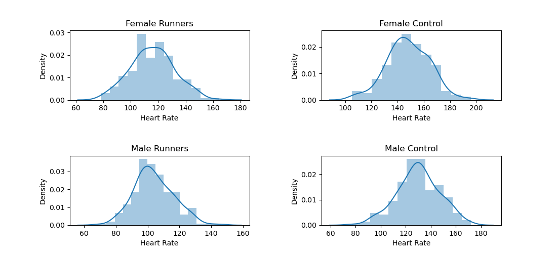
Let's go back to this heart-rate data from Moore, McCabe, and Craig. This dataset contains two factors that vary between subjects (Gender and Group) and one dependent variable (Heart Rate). To test whether Gender, Group, or their interaction affect heart rate, you need the following code.
As above, the combination of ols() and anova_lm() isn't very elegant, but the important part is the formula.
from datamatrix import io
from statsmodels.formula.api import ols
from statsmodels.stats.anova import anova_lm

dm = io.readtxt('data/heartrate.csv')
dm.rename('Heart Rate', 'HeartRate')  # statsmodels doesn't like spaces
df = anova_lm(ols('HeartRate ~ Gender * Group', data=dm).fit())
print(df)
Output:
                 df      sum_sq        mean_sq           F         PR(>F)
Gender          1.0   45030.005   45030.005000  185.979949   3.287945e-38
Group           1.0  168432.080  168432.080000  695.647040  1.149926e-110
Gender:Group    1.0    1794.005    1794.005000    7.409481   6.629953e-03
Residual      796.0  192729.830     242.122902         NaN            NaN
This reveals that heart rate is related to all factors: gender (F = 185.980, p < .001), group (F = 695.647, p < .001), and the gender-by-group interaction (F = 7.409, p = .006).
You can also use the anova function from pingouin.
import pingouin as pg

aov = pg.anova(dv='HeartRate', between=['Gender', 'Group'], data=dm)
print(aov)
Output:
           Source          SS   DF             MS           F          p-unc       np2
0          Gender   45030.005    1   45030.005000  185.979949   3.287945e-38  0.189393
1           Group  168432.080    1  168432.080000  695.647040  1.149926e-110  0.466362
2  Gender * Group    1794.005    1    1794.005000    7.409481   6.629953e-03  0.009223
3        Residual  192729.830  796     242.122902         NaN            NaN       NaN
You can visualize this result with Seaborn:
from matplotlib import pyplot as plt
import seaborn as sns

sns.pointplot(x='Group', y='HeartRate', hue='Gender', data=dm)
plt.xlabel('Group')
plt.ylabel('Heart rate')
plt.show()
Repeated Measures ANOVA
A Repeated Measures ANOVA is generally used to analyze data from experiments in which all participants take part in all conditions, that is, a within-subject design. An example of such a design comes from an experiment by Zhou and colleagues, in which participants searched for a target object in the presence of a distractor object. Either the target, or the distractor, or both could match a color that participants held in memory. You can download this dataset here.
To test whether the factors distractor-match, target-match, and their interaction affect search accuracy, you can use the AnovaRM class from statsmodels.stats.anova.
Somewhat different most other RM-ANOVA software, the AnovaRM class accepts the data in long, unaggregated format. That is, each row corresponds to a single observation. Statsmodels will automatically reduce this format to a format where observations are aggregated per participant and condition (which is the required format for an RM-ANOVA) using the method indicated with the aggregate_func keyword:
from datamatrix import io
from statsmodels.stats.anova import AnovaRM

dm = io.readtxt('data/zhou_et_al_2020_exp1.csv')
aov = AnovaRM(
    dm,
    depvar='search_correct',
    subject='subject_nr',
    within=['target_match', 'distractor_match'],
    aggregate_func='mean'
).fit()
print(aov)
Output:
                           Anova
===========================================================
                              F Value Num DF  Den DF Pr > F
-----------------------------------------------------------
target_match                   6.7339 1.0000 34.0000 0.0139
distractor_match              13.9729 1.0000 34.0000 0.0007
target_match:distractor_match  7.1687 1.0000 34.0000 0.0113
===========================================================
This reveals that search accuracy is affected by all factors: target match (F = 6.7339, p = .0139), distractor match (F = 13.9729, p = .0007), and the target match by distractor match interaction (F = 7.1687, p = .0113).
You can also use the rm_anova function from pingouin.
import pingouin as pg

aov = pg.rm_anova(
    dv='search_correct',
    within=['target_match', 'distractor_match'],
    subject='subject_nr',
    data=dm
)
print(aov)
Output:
                            Source        SS  ddof1  ddof2        MS          F     p-unc  p-GG-corr       ng2  eps
0                     target_match  0.013813      1     34  0.013813   6.733860  0.013863   0.013863  0.002314  1.0
1                 distractor_match  0.013813      1     34  0.013813  13.972917  0.000681   0.000681  0.002314  1.0
2  target_match * distractor_match  0.002136      1     34  0.002136   7.168675  0.011339   0.011339  0.000359  1.0
Let's visualize this result.
We could (but shouldn't!) simply create a pointplot based on dm. But this plot would not take into account that a Repeated Measures ANOVA is based on aggregated data (i.e. one observation per condition and participant). And therefore the error bars of this plot would not reflect the variation between participants (as it should), but rather the variation between individidual trials.
To make a more appropriate figure, we first use ops.group() to create a new datamatrix, gm, in each row corresponds to a single condition for a single participant. Initially, gm.search_correct then corresponds to a series of values, one for each trial. (It is a SeriesColumn, a powerful type of column about which you can read more here.) We use srs.reduce_() to change this series of values to a single, mean value. Finally, we remove the between-subject variability, which is a fancy way of saying that we change search_correct such that it is on average the same for each participant, without changing the overall average of search_correct across participants. (This procedure is described in more detail in this blogpost.)
And then we can finally create a plot that is an appropriate match to the Repeated Measures ANOVA!
from matplotlib import pyplot as plt
import seaborn as sns
from datamatrix import operations as ops, series as srs

# Group the data by condition and subject
gm = ops.group(
    dm,
    by=[dm.target_match, dm.distractor_match, dm.subject_nr]
)
gm.search_correct = srs.reduce_(gm.search_correct)
# Remove between-subject variability
for subject_nr, sm in ops.split(gm.subject_nr):
    gm.search_correct[sm] = sm.search_correct - sm.search_correct.mean + gm.search_correct.mean
# And plot!
sns.pointplot(
    x='target_match',
    y='search_correct',
    hue='distractor_match',
    data=gm
)
plt.xlabel('Target match')
plt.ylabel('Search accuracy (proportion)')
plt.legend(title='Distractor match')
plt.show()
Tip: If you prefer to conduct the RM-ANOVA with different software, such as JASP or SPSS, then you first need to create a so-called pivot table, in which each row corresponds to a subject, and each column to a condition. You can do this with the ops.pivot_table() function:
pm = ops.pivot_table(
    dm,
    values=dm.search_correct,
    index=dm.subject_nr,
    columns=[dm.target_match, dm.distractor_match]
)
print(pm)
Output:
+----+----------+----------+----------+----------+
| #  |   0_0    |   0_1    |   1_0    |   1_1    |
+----+----------+----------+----------+----------+
| 0  | 0.96875  | 0.921875 |    1     | 0.953125 |
| 1  |    1     | 0.96875  |    1     |  0.9375  |
| 2  |    1     |  0.9375  |    1     | 0.984375 |
| 3  |    1     | 0.953125 | 0.96875  | 0.96875  |
| 4  | 0.921875 | 0.859375 |    1     | 0.953125 |
| 5  | 0.984375 | 0.96875  | 0.984375 |    1     |
| 6  |    1     |    1     |    1     |    1     |
| 7  | 0.96875  | 0.96875  | 0.984375 |    1     |
| 8  |    1     | 0.984375 |    1     | 0.984375 |
| 9  |    1     | 0.984375 |    1     |    1     |
| 10 | 0.015625 | 0.03125  |    0     |    0     |
| 11 | 0.984375 |  0.9375  | 0.984375 | 0.953125 |
| 12 | 0.90625  | 0.84375  | 0.953125 | 0.953125 |
| 13 |  0.9375  | 0.984375 | 0.953125 | 0.96875  |
| 14 | 0.828125 |  0.8125  | 0.84375  |  0.8125  |
| 15 | 0.953125 | 0.921875 |    1     | 0.984375 |
| 16 | 0.890625 | 0.84375  | 0.90625  | 0.890625 |
| 17 | 0.984375 | 0.96875  | 0.96875  | 0.96875  |
| 18 | 0.578125 | 0.484375 |   0.5    | 0.515625 |
| 19 |   0.5    |  0.5625  | 0.484375 |  0.5625  |
+----+----------+----------+----------+----------+
(+ 15 rows not shown)
Linear mixed-effects modeling
A linear mixed-effects model (or: linear mixed-effects regression) is a modern statstical-analysis technique for 'hierarchical' datasets. This sounds complicated, but the most common type of hierarchy is simply a dataset that consists of multiple observations from multiple participants. The Zhou et al. dataset, described above, is an example of such a dataset.
In many cases, you can analyze the same dataset using either a Repeated Measures ANOVA or a linear mixed-effects model; however, one crucial difference is that a Repeated Measures ANOVA requires you to aggregate data across multiple observations (e.g. by calculating the mean reaction time per participant and condition), whereas a linear mixed-effects model is performed on unaggregated data, i.e. on individual observations. In addition, linear mixed-effects modeling offers far more flexibility for analyzing complex datasets that you cannot analyze with a Repeated Measures ANOVA.
Let's say that we want to analyze search reaction times as a function of the conditions target match and distractor match, and that we want to have random by-participant intercepts and slopes. The most well-known package for linear mixed-effects modeling is the R package lme4, in which case this analysis corresponds to the formula:
search_rt ~ target_match * distractor_match + (1 + target_match * distractor_match | subject_nr)
In Python, we need to use statsmodels for this, and the syntax is slightly different. Notably, the random effects structure is passed separately as the re_formula keyword:
from datamatrix import io
from statsmodels.formula.api import mixedlm

dm = io.readtxt('data/zhou_et_al_2020_exp1.csv')
model = mixedlm(formula='search_rt ~ target_match * distractor_match',
                re_formula='~ target_match * distractor_match',
                data=dm, groups='subject_nr').fit()
print(model.summary())
Output:
                                 Mixed Linear Model Regression Results
=======================================================================================================
Model:                            MixedLM                Dependent Variable:                search_rt
No. Observations:                 8960                   Method:                            REML
No. Groups:                       35                     Scale:                             105803.2305
Min. group size:                  256                    Log-Likelihood:                    -64683.5652
Max. group size:                  256                    Converged:                         Yes
Mean group size:                  256.0
-------------------------------------------------------------------------------------------------------
                                                       Coef.    Std.Err.   z    P>|z|  [0.025   0.975]
-------------------------------------------------------------------------------------------------------
Intercept                                              1056.900   64.632 16.353 0.000  930.223 1183.577
target_match                                           -113.602   17.267 -6.579 0.000 -147.444  -79.759
distractor_match                                         60.356   11.541  5.230 0.000   37.736   82.976
target_match:distractor_match                            47.132   18.910  2.492 0.013   10.070   84.195
subject_nr Var                                       144553.219  109.235
subject_nr x target_match Cov                         -1867.445   20.680
target_match Var                                       7128.699    7.796
subject_nr x distractor_match Cov                     -3217.240   14.003
target_match x distractor_match Cov                   -2778.028    3.725
distractor_match Var                                   1355.484    3.482
subject_nr x target_match:distractor_match Cov         2470.514   22.659
target_match x target_match:distractor_match Cov       -109.659    6.291
distractor_match x target_match:distractor_match Cov    377.434    4.315
target_match:distractor_match Var                      5902.857    9.349
=======================================================================================================
This reveals that search reaction times are affected by all factors: target match (z = -6.579, p < .001), distractor match (z = 5.230, p < .001), and the target match by distractor match interaction (z = 2.492, p = .013).
Exercises
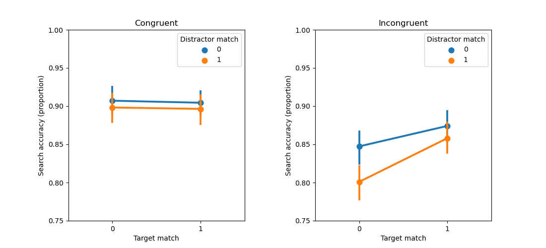
A three-way Repeated Measures ANOVA
Above you have seen how to conduct a two-way repeated measures ANOVA with this dataset from Zhou et al. (2020). But the data contains a third factor: congruency. First, run a three-way repeated measures ANOVA with target-match, distractor-match, and congruency as independent variables, and search accuracy as dependent variable. Next, plot the results in a two-panel plot, where the left subplot shows the effect of distractor and target match for congruent trials, while the right subplot shows this for incongruent trials.
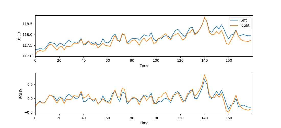
Correlating activity in the left and right brain
- Read this dataset, which has been adapted from the StudyForrest project. See Exercise 2 from the NumPy tutorial if you don't remember this dataset!
- Get the mean BOLD response over time, separately for the left and the right brain.
- Plot the BOLD response over time for the left and the right brain.
- You will notice that there is a slight drift in the signal, such that the BOLD response globally increases over time. You can remove this with so-called detrending, using
scipy.signal.detrend(). - Plot the detrended BOLD response over time for the left and the right brain.
- Determine the correlation between the detrended BOLD response in the left and the right brain.
Statistical caveat: Measures that evolve over time, such as the BOLD response, are not independent. Therefore, statistical tests that assume independent observations are invalid for this kind of data! In this exercise, this means that the p-value for the correlation is not meaningful.
You're done with this section!
Continue with Time series >>